AMI Analysis

The AMI Analysis dialog allows you to perform AMI analysis for a target signal. The analysis using the IBIS-AMI model specifies the dedicated stimulus, and adjusts the parameters that are provided by the model. Launch this dialog by clicking Tool > AMI Analysis on the main menu in Electrical Editor.

Target Signal Table

Item		Description
Signal		Displays the name of the signal to be analyzed.
AMI Stimulus		Displays the AMI stimulus that is assigned to the signal. To assign an AMI stimulus to a signal, point the cursor in this cell and then click the displayed button. The AMI Stimulus dialog is displayed. Select an AMI stimulus name from the file list, and click OK. The AMI stimulus is assigned to the signal, and the following values are displayed.
	Bit Pattern	Displays the digital stimulus pattern that you specify for the stimulus. This is typically a Pseudo Random Bit Sequence (PRBS) with a relatively large number of bits, and a particular data rate. Alternatively, a periodic Clock signal could be used to drive the serial channel. This value is specified in the AMI Stimulus dialog.
	Data Rate	The data rate of the Clock signal or PRBS sequence that drives the serial channel. This value is specified in the AMI Stimulus dialog. It should be set according to the data sheet for the model.
	Bit Order	Specifies the length of a PRBS stimulus. This value is specified in the AMI Stimulus dialog. If you specify a Clock signal in the AMI Stimulus dialog, Bit Pattern field, then a value is not shown in the Bit Order column.
	Encoding	If you select PRBS in the AMI Stimulus dialog, Bit Pattern field, then the encoding scheme is shown that you select for the data transmission. This is specified in the AMI Stimulus dialog, Encoding field.

Property Table

Transmit and receive values are shown in the Tx and Rx columns, respectively, for the relevant scenario.

Item	Description
Reference	Displays the Reference designator values of the pin to be analyzed.
Differential Pins	Displays the pin numbers of the differential pins to be analyzed.
Buffer Model	Displays the name of the buffer model that you assign to the pin in the Select Model dialog. This is launched by right-clicking the pin on the canvas and then selecting Assign Model.
AMI Architecture	Information is displayed regarding the AMI model that is assigned to the pin. This is defined as a sub parameter of Algorithmic Model in the IBIS model. See: AMI Models for TX and RX.
AMI Executable File	Shows the name of the AMI Executable File. This is a binary executable file for AMI analysis that is located within a shared library.
AMI Parameter File	The model makers provide AMI parameter (.ami) files as well as executable files, in order to configure the algorithmic model behavior in the run-time library. You can edit the AMI parameter files in order to control the behavior of the algorithmic model. Output parameters can be modified by the algorithmic model during the analysis. The available AMI parameters and their allowed value ranges are provided in the AMI parameter file, with a set of default values. You can configure the sets of parameters in the AMI Parameters dialog.
AMI Parameter Set	Displays the name of the AMI parameter set. This is specified in the AMI Parameters dialog. Launch this dialog by pointing the cursor in this cell, and then clicking the displayed button. If no AMI Parameter Set is specified, then <Default> or <Jitter> is displayed.
Size of Data Sequence	Displays the length of the data sequence that is used to divide the number of bits. The allowable range is 1,024 to 10,485,760. If no data sequence length is found, then 1024 is displayed.

Channel Characterization

This section allows you to perform Channel Characterization. The analog channel characterization is performed in the Frequency Domain. This initial step must consider the intended data rate of the serial link, using an appropriate frequency range. The upper frequency range must not be lower than the intended data rate. See: AMI Analysis Flow.

Item	Description
Maximum Frequency	Specify the upper frequency limit of the simulation frequency. This is related to the Time-Domain resolution that is used to derive the impulse response function h(t). The allowable range is 100 MHz to 500 GHz. The Data Points field is automatically updated when you enter a value.
Equidistant Frequency Step	Specify the equidistant step value in all frequency bands. This value relates to the overall duration of the impulse response function. To obtain accurate results, the frequency sampling must be sufficiently dense. The allowable range is 100 kHz to 100 MHz. The Data Points field is automatically updated when you enter a value.
Data Points	Shows the number of points to calculate. This value is produced by dividing Maximum Frequency by Equidistant Frequency Step, and then adding "1". The first point is "0.0". For example, for a Maximum Frequency of 100 MHz and an Equidistant Frequency Step of 25 MHz, the following frequencies are calculated: 0.0 MHz 25 MHz 50 MHz 75Mhz 100MHz . The Data Points value is updated automatically when you enter values in the Maximum Frequency and Equidistant Frequency Step boxes.
Causality Enforcement	In some cases, for example when a lossy transmission line (TL) model is used, the channel characteristic may become non-causal. A non-causal S-Parameter data set, which is used as part of the channel, may also be a cause of causality violations. Select this check box to correct this. Note It is recommended to , check the S-Parameter data for causality before using them in AMI Analysis.
Ignore IC Package	IBIS buffer models may come with an assigned package model. This simple package model may interfere with a more detailed package model, provided by S-Parameters for example. If Ignore IC Package is selected, then the IBIS IC package is ignored in the analog channel. Note Channel characterization can be performed with non-IBIS AMI models (legacy IBIS models) assigned in the scenario.

Channel Characterization Results

The results of the channel characterization values that you set in the AMI Analysis dialog can be viewed using the following methods. The results are in the Time Domain and Frequency Domain. Each result provides useful information about the quality of the interconnect. Potential problems within the layout geometry may become visible by inspecting the impulse response or the transfer function, for example.

Value		Description
S-Parameter		Allows you to inspect the analog channel characteristics as a set of S-Parameters. The frequency range and frequency stepping are controlled by the respective settings. Note The calculated S-Parameters contain only the analog channel (which may include the IBIS IC package model), but without the analog part of the RX/TX model. The S-Parameter data can therefore be transferred to other tools for further channel analysis. Use the CSV Export command in Analysis Result Viewer.
	View	Calculates the S-parameter, and launches the Analysis Result Viewer. Example results are shown below.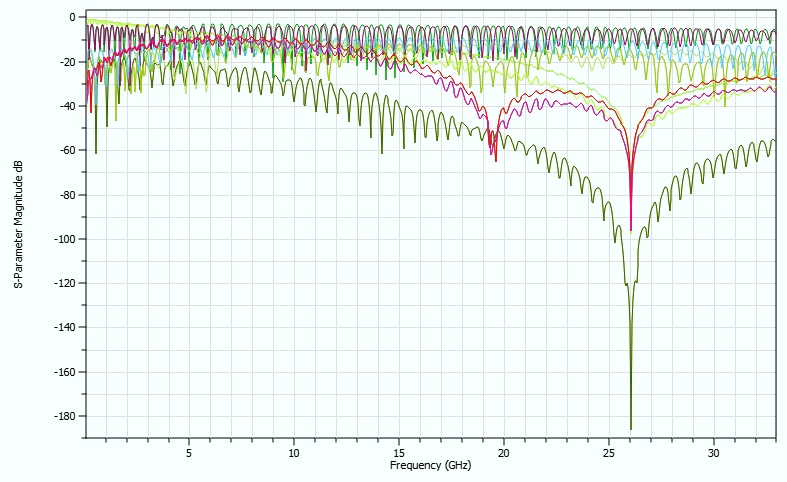
Transfer Function		The channel’s transfer function H(f) in the Frequency Domain is another measure for the quality of the impulse response function. The frequency range and frequency stepping are controlled by the respective settings. If the transfer function H(f) still shows a significant magnitude at the upper frequency range of the analyzed spectrum, then the involved numerical methods may cause an unwanted alteration of the applied transfer function.
	View	The Analysis Result Viewer is launched. This displays the transfer function H(f) in the specified frequency range. Example results are shown below.
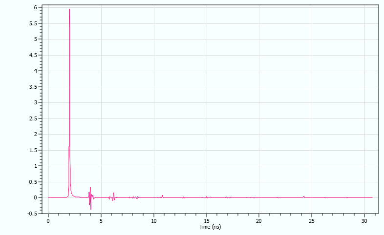
Impulse Response		The impulse response function h(t) is the primary input into the AMI model. This function is essential to the quality of the resulting eye pattern. Therefore, any signal distortion due to an insufficient frequency range should be avoided as much as possible. It is recommended that the impulse response function has settled within the simulation time.
	View	The Analysis Result Viewer is launched. This allows you to visually inspect the impulse response function h(t). Example results are shown below.

AMI Simulation

The AMI Simulation section allows you to specify the following analysis conditions.

Item		Description
Number of Bits to Simulate		Allows you to specify the number of bits to simulate, within the range 2⁸ to 2³⁶. Specifying the number of bits to simulate will affect the total AMI Analysis time to generate an Eye Pattern. In order to predict a meaningful Bit Error Ratio (BER), a significant number of bits must be simulated. Based on these calculated bits, the BER is extrapolated using statistical methods which exploit Jitter data on the channel. A BER of 10-15 is the lowest value that is possible in eCADSTAR.
	Units	Select the required units. The following units can be selected. bit kbit Mbit Gbit
Number of Bits to Skip		Specify the number of leading bits to skip, between 0 and the Number of Bits to Simulate value. The connected AMI models require initialization procedures to set up the internal digital filter and pre-emphasis parameters. Consequently, a required number of bits must be skipped from the Eye Pattern analysis, and correspondingly from the BER prediction. Check the model documentation for a meaningful value for this parameter. You can view the initialization process in the time-domain waveform of the AMI Analysis.
	Units	Select the required units. The following units can be selected. bit kbit Mbit Gbit
Sampling Rate per Bit		Determines the time resolution of the resulting Eye Pattern. A higher value improves the resolution, but leads to increased analysis times and memory requirements. The allowable range is 8 to 128.
Probe Position		Allows you to select the position within a serial channel that is used to probe for an Eye Pattern. The Tx In probe represents just the stimulus. Consequently, only an ideal rectangular “eye” can be computed. This is not provided in eCADSTAR. To open the eye pattern, digital signal processing at the driver and receiver side is applied. A pre-emphasis of some dB improves the eye opening by strengthening the low-to-high and high-to-low transitions at the driver side (TX). The AMI parameter settings (for example, for equalization) for the driver (TX) and receiver (RX) can be specified in the AMI Parameters dialog. Refer to the model maker's documentation for information on the available parameters, and recommended settings. Note If no IBIS AMI models are assigned to the driver and receiver buffer, then an Eye Pattern can still be computed using the channel’s impulse response functions, and the input stimulus pattern. In this case, only the Rx Out probe position can be shown. If an IBIS AMI model is assigned to the receiver buffer only, then the RX In probe becomes available, as well as the Rx Out probe. If an IBIS AMI model is assigned to the driver buffer only, then the TX Out probe becomes available, as well as the Rx Out probe.
	Tx Out	If selected, then the output of the AMI part of the driver model is measured. This probe shows the impact of the TX model settings.
	Rx In	If selected, then the input of the AMI part of the Rx (receiver) model is measured. This probe frequently shows a slightly closed eye pattern caused by dispersion, discontinuities and losses in the transmitting channel. This frequency-dependent attenuation causes significant inter-symbol interference (ISI) in the received signal. This causes difficulty for clock and data recovery, and causes a high bit-error rate (BER).
	Rx Out	If Rx Out is selected, then the output of the AMI part of the Rx (receiver) model is measured. At the receiver end (RX), equalization aims for a better overall (flat) transfer function. This removes the impact of the channel. The Rx Out probe shows the Eye Pattern behind this stage. Note The Rx Out value cannot be measured if any of the following apply to the Rx (receiver) model. An existing IBIS model is assigned to it. No AMI executable file exists. No AMI parameter file exists.

Continuous AMI Waveform

Value		Description
Length of Waveform		Allows you to specify the number of bits that are simulated. The allowable range is 8 to 1024.
Waveform
	View	Displays the waveforms in which leading bits are skipped, as specified in the Number of Bits to Skip field. The Analysis Result Viewer is launched.

Value	Description
Execute	The AMI analysis is executed, and the Analysis Result Viewer is launched. If the Tx / Rx model is an existing IBIS model, then an eye pattern is generated on the basis of impulse response. Analysis results can be viewed in Continuous AMI Waveform.
Close	The AMI Analysis dialog is closed. The changed AMI stimulus assignment, AMI parameter set and analysis conditions are saved.

Note

It is recommended that you select an AMI architecture that is suitable for your operating environment.
Multiple signals cannot be analyzed.
The AMI Analysis dialog can only be opened when a buffer model is assigned to the pin.
Different types of executable file are defined in the IBIS-AMI model, such as "Platform","Compiler" and "Bits". This depends on the environment in which the executable file is created.

Related Topics
AMI Analysis: Introduction