The main window of the Analysis Result Viewer allows you to examine analysis results data. It comprises the following main areas.
Menus and Toolbars allow you to access the functions of the application. Shortcuts to functionality are also provided.
You can re-arrange content in the main window by dragging the elements, either within their frame or outside of it. The basic layout of the main window is shown below.
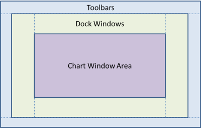
Within an outer frame, the toolbars can be re-arranged and docked at any position by easily dragging them around. Inside this area, you can place dockable windows around the central Chart Window Area. Multiple dockable windows at the same location are displayed using tabs. Select the required tab to display it foremost.
The actual Chart Windows are displayed within the Chart
Window Area. They are displayed either as a single window, a tiled layout
next to each other or they are cascaded on top of each other. The following
toolbar icons allow you to control the display style of the Chart Windows:
Tiled  or Cascaded
  .
.
Each Chart Window can host several individual charts:
electric fields, impedances, voltages, currents and stimulus in both time
and frequency domain. Filter buttons allow
you to quickly create a required view: for example, for voltage charts in the time domain
  .
Depending on the content of the loaded data sources, the filter buttons
may be active or inactive.
.
Depending on the content of the loaded data sources, the filter buttons
may be active or inactive.
When you close the Analysis Result Viewer, the current layout and other settings are saved in the APPDATA\Roaming\Zuken\eCADSTAR{version}\Analysis\Settings\viewer.ini file. You can also define up to three layout views which can be saved and restored at any time. Use the View menu entries to load and save layouts.
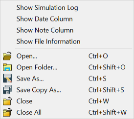
To control the visible elements, right-click any frame or empty toolbar area and select from the following items on the assist menu.
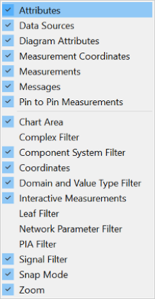
The items that are displayed depend on the available elements in the current operation mode.
The following numbered areas in the main window are described below.
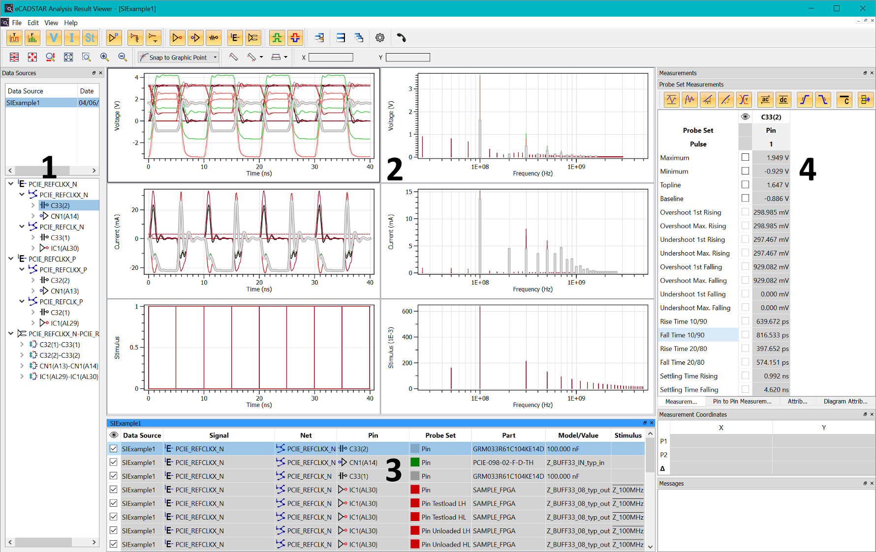
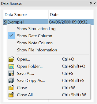
1: Data Sources Area
The Analysis Result Viewer can handle a variety of Data Sources of different types.
Multiple data sources of the same type can be loaded into the same instance of the Analysis Result Viewer. These are shown in the Data Sources area.
When opening a different type of data source such as SI Eye Pattern results within the regular SI data context, a new instance is opened to display the SI Eye Pattern.
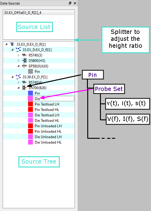
The Data Sources area comprises a source list and a source tree beneath the list. Use the splitter bar to adjust the relative sizes of the list and tree size. The source list shows all opened data source files, in the order in which they are opened.
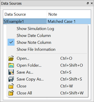
You can enter a note next to an opened data source to annotate it. This allows you to differentiate between different analysis cases. In the case of an srdb file, the note is stored with the data source file when it is closed. Other file types, such as Touchstone files are not modified, and no note is stored.
For the SI Parameter Sweep data source, you can expand the list entry to show the set of individual SI simulations.
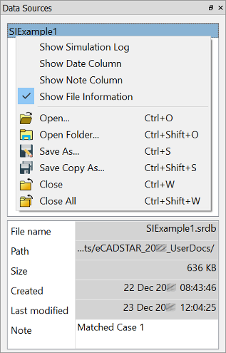
- The assist menu gives you quick access to some
functions which are also available on the File
menu. This is accessed by right-clicking in the Data Sources area,
or using the shortcut keys.
| Value | Description | Shortcut |
|---|---|---|
 Open Open
|
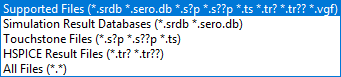
Allows you to open a data source file, or another data source file if data source files are already open. Data source files are generated by the SI Simulation System, or the PI/EMI Analysis module. A file selection dialog is opened. Select the data source file to be opened and click Open. Alternatively, click Cancel to cancel the operation. When opening a data source which is a different type to the currently-loaded one, a new instance of the Analysis result Viewer is opened. See the Data Source section for details on the types of data sources. The file browser allows to filter for a supported file type.
If you try to open an unsupported file type, then a warning message is displayed and the file is not loaded. |
Ctrl+O |
 Open Folder Open Folder
|
Open more than one data source by opening a folder containing multiple data source files. | Ctrl+Shift+O |
 Save As Save As
|
Save the selected data source file in a new file (location) with a new name. Any changes made to the data source will be saved to this new file. Its name is updated in the Data Source List to the name that you specify. | Ctrl+S |
 Save Copy As Save Copy As
|
The selected Data Source is saved in a new file location as a duplicate file. The name of the selected Data Source is not changed. | Ctrl+Shift+S |
 Close Close
|
Closes the selected data source, and removes its content from the Chart area and the related Working Sets. If there are unsaved changes, then a confirmation dialog is displayed. Click Save to save the changes. Alternatively, click Cancel to cancel the operation or click Discard to discard the changes. |
Ctrl+W |
 Close All Close All
|
Close all data source files that are currently open. | Ctrl+Shift+W |
The source tree displays the content of the
selected entries in the source list, in an hierarchical tree view. After
loading a new data source by clicking  , this data is
shown in the source tree.
, this data is
shown in the source tree.
Typically, a new Working Set is created for each loaded data source. It's chart content is displayed in the Chart area.
The Settings dialog allows you to control the behavior of Working Sets when loading new data sources. For example, to add probe sets into an existing Working Set. When selecting a data source, the related Working Set with the same name is also selected.
The source tree contains nodes for each data object. For
example, component pin. The type of node is indicated by an appropriate
icon, such as a receiver pin  .
A table of the symbols that are used is provided here.
.
A table of the symbols that are used is provided here.
Probe Sets in SI Analysis
Each leaf may represent one or more charts. For example, voltage against time and current against time. This group of charts is called a "Probe Set". These are defined by the probing location, and the data domain type, which could be time or frequency.
In addition to the chart data, various attributes and measurement data are contained in a probe set. The actual content depends on the node type.
Example
A driver pin's list of probe sets may contain the following entries.
- Chart data at Pin location in the time domain (voltage and current).
- Chart data at Die location in time domain (voltage and current)
- Chart data at Pin location in the frequency domain (voltage and current)
- Chart data at Die location in frequency domain (voltage and current)
- Chart data for test Load condition at Pin location (L-H and H-L transition)
- Chart data for test Load condition at Die location (L-H and H-L transition)
- Chart data for open condition at Pin location (L-H and H-L transition)
- Chart data for open condition at Die location (L-H and H-L transition)
- Chart data for stimuli.
- Attributes for Chart drawing style (color, line width, line type)
- Automatic measurement results derived by the analysis kernel
The drawing attributes are common for all chart data within one probe set. They can be controlled in the Working Set area.
Define different color sets in the Settings dialog for the different probe set types. These are used when loading data sources into the Analysis Result Viewer.
Probe Sets in EMI and PI Analysis
In PI and EMI mode, the used probe sets contain fewer individual charts than in the SI modes. The probe sets depend on the PI/EMI Analysis result types, and may contain the following entries.
- Chart data for Total Radiation
- Chart data for Signal Loop Radiation
- Chart data for I/O Driven By Radiation
- Chart data for Heatsink related Radiation
- Chart data for Connector related Radiation
- Chart data for Power Bus Radiation
- Chart data for Impedances (Magnitude and Phase)
- Chart data for Voltages
- Combined Chart data, depending on suitability. For example, for radiation from multiple selected E-Nets. This information is generated by the EMI and PI Analysis System, and cannot be calculated within the Analysis Result viewer.
- Attributes for Chart drawing style (color, line width, line type).
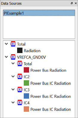
The different types of probe set are identified by the specific symbols shown below.
The data sources are generated automatically by the PI/EMI Analysis module in separate files. By moving them into a single Working Set, you can compare different probe sets within one Chart. No automatic measurement results are stored with the probe sets for any EMI and PI results. The Measurements window therefore remains empty in the EMI and PI mode.
Probe Sets for S-Parameters
S-Parameters are defined for single-ended or differential ports. Respective Probe Sets are available within the Data Sources view. Their type is either Standard S, or Mixed-mode S-Parameters.
 Each single-ended, standard
S-Parameter port
Each single-ended, standard
S-Parameter port  is described by its port
number, for example, "SP1", and the related component pin name.
In addition, the probe location is identified by Pin
or Die. For each port "i",
the S-Parameters are listed to all other ports (Sij), and the reflection
parameter at the port itself (Sii). The probe sets are named P<i.j>.
is described by its port
number, for example, "SP1", and the related component pin name.
In addition, the probe location is identified by Pin
or Die. For each port "i",
the S-Parameters are listed to all other ports (Sij), and the reflection
parameter at the port itself (Sii). The probe sets are named P<i.j>.
 if mixed-mode S-Parameters
are present, then the differential ports
if mixed-mode S-Parameters
are present, then the differential ports  are
described with their differential port number, for example, "DP1",
their single ports and their related component pin names of the differential
pin pair. For example, "IC1(A2) - IC1(A4)".
are
described with their differential port number, for example, "DP1",
their single ports and their related component pin names of the differential
pin pair. For example, "IC1(A2) - IC1(A4)".
The Probe Sets are listed for each port with their relationship to the following modes.
- DD Differential-Differential-mode
- DC Differential-Common-mode
- CD Common-Differential-mode
- CC Common-Common-mode
The probe sets for mixed-mode S-Parameters are named P<cd><i.j>.
When single-ended ports are combined with differential ports, the relation between the differential and single-ended ports are listed in the mixed-mode part of the tree. In this particular case these additional probe sets are available.
- DS Differential mode-Single
- CS Common mode-Single
- SD Single-Differential mode
- SC Single-Common mode
- SS Single-Single
A Probe Set for S-Parameters contains charts for magnitude
and phase. Use the toolbar icons  and
and  to
control the display of these charts.
to
control the display of these charts.
Mixed-mode S-Parameters are derived automatically from the Standard S-Parameters, when differential pin pairs are detected in the data source.
This functionality is not available for Touchstone V1 imported data.
Used Symbols
| Symbol | Element type |
|---|---|
|
|
E-Net level |
|
|
Differential Pair level |
|
|
Tri-State driver pin |
|
|
Driver pin |
|
|
Bi directional driver pin |
|
|
Receiver Pin |
|
|
Bi directional receiver pin |
|
|
Tri-State high impedance |
|
|
Capacitor |
|
|
Inductor |
|
|
Diode |
|
|
Resistor |
|
|
Connector pin |


EMI and PI specific symbols
| Symbol | Element type |
|---|---|
|
|
IO Net Emission |
|
|
Signal Loop Emission |
|
|
Net Total Emission |
|
|
Connector Board Emission |
|
|
Connector Heatsink Emission |
|
|
Connector Connector Emission |
|
|
Connector Total Emission |
|
|
Heatsink Board Emission |
|
|
Heatsink Connector Emission |
|
|
Heatsink Total Emission |
|
|
Common Mode Voltage |
|
|
Power Bus Emission |
|
|
Power Bus Noise Voltage |
|
|
Supply System or Power Bus |
|
|
Supply Pin |
|
|
Position |


S-Parameter Symbols
| Symbol | Element type |
|---|---|

|
Standard S-Parameter |

|
Mixed-mode S-Parameter |

|
Single-ended Port |

|
Differential Port |
Other Symbols
| Symbol | Element type |
|---|---|
|
|
Transfer Function |
|
|
Impulse Response |
2: Chart Window Area
The Chart window area allows
you to view the actual charts. Multiple Chart
windows can be shown, and arranged in various ways. For example, Tiled
or Cascaded .
Each Chart window is related to a Working Set. This is a group of charts which is displayed together in one Chart window. Therefore, the Chart Window and Working Set always appear as a pair. The title of the Chart window is the name as the working set: "Set <number>". See: Working Set Area.
You can create your preferred arrangements by moving and
re-sizing the individual Chart windows.
Use the maximise  button, or double-click the window
title to maximize the Chart window within
the Chart window area.
button, or double-click the window
title to maximize the Chart window within
the Chart window area.
Within each Chart window, several charts can be created, as described below. A fixed table layout of rows and columns is used to arrange these by their specific type within each of the Chart Windows.
Specify which of these charts is shown using the following
filter buttons
on the toolbar: 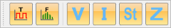
Assist Menu
The following options are displayed on the assist menu by right-clicking in a Chart window.
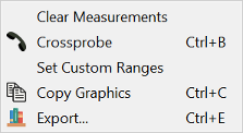
| Value | Description |
|---|---|
| Clear Measurements | Removes all measurement lines from the chart display. This action also clears the display in the Measurement Coordinates window. |
 Crossprobe Crossprobe
|
Allows you to cross-probe the selected item with other applications, such as eCADSTAR PCB Editor and PI/EMI Analysis Module, selecting the relevant item on the canvas in. Alternatively, press Ctrl+B. Note
The cross-probing only works from Electrical Editor to Analysis Results Viewer. The Electrical Editor will not process cross-probing requests from Analysis Results Viewer. |
| Set Custom Ranges | Applies the current zoom ranges of the active Chart window to the axis ranges in the Diagram Attributes windows. This function provides a graphical method to set the axis ranges in addition to the manual one. |
 Copy Graphics Copy Graphics
|
Copies the currently selected chart window to the clipboard. |
 Export Export
|
Displays the Export dialog. This allows you to store results data in either CSV or image format. |
Controlling the Display of Charts
You can use the Domain Type Filter
buttons for Time  or Frequency
  Domain plots in both columns.
The Value Type Filter buttons
for voltage  , current
  , and stimulus
 enable
the display of the corresponding charts, arranged in rows on top of each
other.
enable
the display of the corresponding charts, arranged in rows on top of each
other.

If more than one row is enabled, the horizontal axes are synchronized with each other when zooming or panning the Chart.
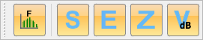
Further
result types in the PI/EMI
mode are: Electric field strength  ,
Impedance
,
Impedance ![]() , and relative
voltages in dB
, and relative
voltages in dB .
.
When S-Parameter data are loaded, specific
toolbar icons are also available. For example,  .
.
You must select as these are all frequency domain results.
Zooming and Panning a Chart
In addition to the toolbar buttons for zooming, you can use the keyboard or a wheel mouse to control the view of a chart. Select the chart to change its view. The supported shortcuts are listed here.
Panning
You can move the visible chart area in the respective direction using the up, down, left and right arrow keys. Alternatively, use the middle mouse button to drag the view.
Zooming
- Use the + or - keys to zoom within a selected chart.
These keys correspond to the
 and
and  buttons. Alternatively,
use the wheel mouse to zoom in and out. Use the current mouse position
as the focus point of the zoom action.
buttons. Alternatively,
use the wheel mouse to zoom in and out. Use the current mouse position
as the focus point of the zoom action. - The Shift key allows you to modify the vertical axis of the just the selected chart.
- The Alt key allows you to modify just the horizontal axis.
- The W key zooms
all charts so that they are visible within the selected Chart area.
This action is equivalent to pressing the
 button.
 - Pressing Shift+W adjusts all charts for the selected working
set. This action is equivalent to pressing the
 button.
 - The Z key invokes
the Zoom Area action. This action
is equivalent to using the
 button. In the Zoom Area mode,
you can define a rectangular area by dragging the cursor.
button. In the Zoom Area mode,
you can define a rectangular area by dragging the cursor.
Custom Zoom
All enabled custom axis settings are applied by clicking
the  -button or by pressing
Shift+C.
Define the custom axis ranges and the scale type in the Diagram
Attributes window.
-button or by pressing
Shift+C.
Define the custom axis ranges and the scale type in the Diagram
Attributes window.
When displaying multiple related charts in the time domain within one Chart window, they keep the same horizontal axis when zooming or panning the view. Charts could include voltage, current or stimulus waveform.
3: Working Set Area
What is a Working Set?
A Working Set contains a group of probe sets which are displayed within one Chart window. The Working Set and Chart window appear as a pair, in which selections are linked together. The name of the Working Set for automatically created working sets on opening a data source is derived from the opened data source.
- If you create new working
sets using the toolbar icon
 , then the
name is defined automatically.
, then the
name is defined automatically. - Use the Settings dialog to control the behavior of Working Sets when loading new data sources. For example, to add probe sets into an existing Working Set.
- The Working Set entries are cross-selected from the Data Sources tree view.
- The Working Set area lists all contained probe sets, and shows important related information.
- The Working Set area cannot be edited. However, you can change the color and line style attributes in the Attributes window, for the selected entries.
Columns of the Working Set
SI related data sources show the following content.
When using a Parameter Sweep data source, the working set contains a set of columns which list the varied parameters. For example, the value of a resistor or a transmission line length. These columns are added to the end of the table, and are indicated with a light blue background color.
The Working Set S-Parameters lists the ports for each data source. The Network Parameter column refers to standard S-Parameters or Mixed-mode S-Parameters.
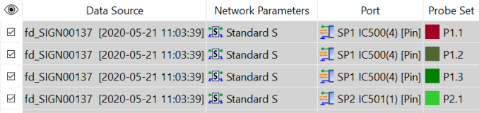
The Port column lists the port name, and the related component and pin name. It also shows the probe location as Pin or Die.
Probe Set refers to the matrix element Sij.
In SI Eye Pattern mode, the Working
Set indicates the currently selected Base
Signal, by showing a modified icon including a "B" on the
selected Base Signal probe:  .
Right-click and choose Set Base Signal
on the assist menu to select the base signal for the Eye Pattern display.
Alternatively, double-click or press the B
key. The base signal defines where the Eye Pattern is centered. All other
probes are displayed relative to this base signal.
.
Right-click and choose Set Base Signal
on the assist menu to select the base signal for the Eye Pattern display.
Alternatively, double-click or press the B
key. The base signal defines where the Eye Pattern is centered. All other
probes are displayed relative to this base signal.
Changing the base signal may take a long time, especially when large eye pattern data are loaded.
The actual Eye Pattern diagram is re-generated from the time domain simulation result, and the Eye Pattern measurement data are recalculated as well.
Select Set Strobe Signal
on the assist menu to select the Strobe Signal for the Setup and Hold
measurement.
The Working Set indicates the currently selected Strobe Signal, by showing
a modified icon including an "S" on the selected probe: 
AMI Eye Pattern and AMI Time-Domain waveforms are based on a specific analysis flow, which is capable of simulating very long bit pattern. This produces Eye Pattern directly as a two-dimensional histogram chart for an AMI model. Hence, no Strobe Signal or Base Signal can be specified for an AMI Eye Pattern. The Time-Domain waveforms can be handled as any other SI waveform. No SI Measurement values are obtained in the AMI Analysis.
AMI File
The AMI file containing the executable model used within the AMI Analysis is listed here.
Parameter Set
The name of the AMI Parameter Set used in the AMI Analysis
is listed here. Click ![]() to open
the AMI Parameters
dialog for viewing the used parameters. An overview of the AMI Parameters
is also available in the dockable AMI
Parameters window. Select AMI
Parameters from the assist menu to view the AMI parameters for the selected AMI model
Probe Set.
to open
the AMI Parameters
dialog for viewing the used parameters. An overview of the AMI Parameters
is also available in the dockable AMI
Parameters window. Select AMI
Parameters from the assist menu to view the AMI parameters for the selected AMI model
Probe Set.
EMI and PI related data sources only use a subset of information listed in the Working Set. The EMI and PI Working Sets may contain Probe Sets called "Combined". These are calculated as a combination of multiple selected items (For example, E-Nets) in the PI/EMI Analysis module.
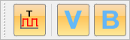
- Use the filter button
 to enable or disable these types of probe sets.
 - Use
 to toggle the display of individual probe sets.
 - Define different color sets in the Settings dialog for the different types of probe set. These are used when loading data sources into the Analysis Result Viewer.
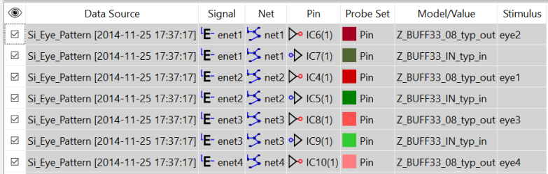
 Visibility
The Visibility check box controls the display of the probe set in the Chart area.
Data Source
This column is only visible when multiple different data sources are contained within the source list. This clearly identifies the probe set by showing the Data Source Name.
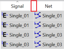
Signal
Provides the name of the E-Net or Differential Pair signal.
Pin
Displays the name (reference designator) of the component. The pin name is shown in brackets. For example, "D1 (A13)".
Part
Shows the part name of the related component.
Probe Set
The type of probe set and its color is shown in this column. In PI /EMI mode, the probe set depends on the analysis context and may contain the following.
- Signal Loop Radiation
- Total Signal Loop Radiation
- I/O Driven By Radiation
- Power Bus Radiation
- Noise Voltage
- Common Mode Voltage
For Impedances
- POW <Power Plane Layer No.> GND <Ground Plane Layer No.>
- Parallel Circuit of the above
- Impedance
For decoupling capacitors (decaps):
- Impedance (Mounted)
- Impedance (ESL)
In AMI Eye Pattern mode,
the Probe Set describes the probing location within the series channel
at the Transceiver (TX) and the Receiver (RX) side.
This may contain:
- TXin and TXout
- RXin and RXout
Eye Patterns are typically available for the RX out probe location, after the digital signal processing within the receiver component.
The following Probe Set types are supported in SI Analysis:
- Pin
- Die
- Pin Unloaded with actual stimulus
- Die Unloaded with actual stimulus
- Pin Testload with actual stimulus
- Die Testload with actual stimulus
- Pin Unloaded Low-High transition, and Pin Unloaded High-Low transition
- Die Unloaded Low-High transition, and Die Unloaded High-Low transition
- Pin Testload Low-High transition, and Pin Testload High-Low transition
- Die Testload Low-High transition, and Die Testload High-Low transition
The Testload and Unloaded waveforms are used to derive Compensated Flight Time measurements at a receiver pin, relative to a given driver pin into test load condition. These reference simulations against test load conditions are well-defined by the driver model data, and require pre-defined stimuli for the driver: a single Low-High, and a single High-Low transition. For additional information, see: Appendix.
Model/Value
Additional information related to the Pin is shown here. This includes the buffer model name, or the value of a passive component.
Stimulus
Shows the base name of the stimulus file.
Description
Shows additional information on the probe set.
Actions within the Working Set
Sort all columns of the Working Set by clicking into the column header. Repeated clicking reverses the sort order.
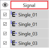
Resize the columns by either double-clicking on the cell splitter for optimal width. Alternatively, move the cell splitter between two columns. The row height cannot be modified.
You can change the order of columns by dragging a column header to another position within the header bar of the Working Set.
The Working Set window can be rearranged within the docking area or even outside of the main window, on the desktop of your PC.
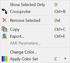
Working Set: Assist Menu
The following options can be selected by right-clicking and selecting them on the assist menu.
| Value | Description |
|---|---|
| Show Selected Only | Shows only the selected probe. Alternatively, press D. To show all probe sets, select all probes and perform the same action. Alternatively, press Ctrl+A and then press D. The Visibilitycheck box also allows you to control the visibility of a Probe Set. |
| Crossprobe
|
Allows you to cross-probe the selected item with other applications. See Crossprobe in the section above. |
|
|
Allows you to remove selected Probe Sets
from the Working Set and the related Chart
Window. Alternatively, press the Delete key. |
| Copy
|
Copies the selected rows of the Working Set to the clipboard.
Alternatively, select Ctrl+C. This allows you to paste it into
other applications, such as MS
Excel.
Note The Visibilitycolumn is not copied to the clipboard as it has no relevance outside of the Analysis Result Viewer. However, the column header information is added automatically. |
| Export
|
Displays the Export dialog. Alternatively, press Ctrl+E. This allows you to export the working set to a CSV or image file. |
| AMI Parameters |
View the AMI parameters for the selected AMI model Probe Set. See AMI Analysis: AMI Parameters Dialog. |
| Change Color | Changes the color of the Probe Set. Alternatively, press the |
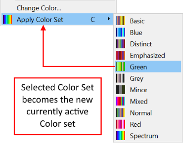
 Apply Color Set Apply Color Set
|
Allows you to change the color set for the selected probe
sets. This also changes the currently-active color set, which
can be used by the "C" shortcut. This immediately applies
the indicated Color Set.
For Example, you can change the color of all driver pins in order to gain a better differentiation of the waveforms. Do this by selecting all probe sets using the Ctrl or Shift key, and then right-clicking and selecting Apply Color Set on the assist menu. |

In Eye Pattern mode, the following context menu is shown.
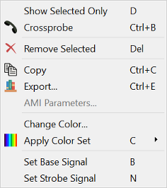
| Value | Description |
|---|---|
| Set Base Signal | Defines the base signal for Eye Pattern display, and is available only in the Eye Pattern mode. Alternatively, press B. |
| Set Strobe Signal | Defines the strobe signal for Eye Pattern display, and is available
only in the Eye Pattern mode.
The strobe signal is applied in Setup and Hold measurements.
|
Creating new Working Sets
Working Sets are created automatically when loading a
new Data Source into the Analysis Result Viewer. It is also possible to
create a new Working Set using the toolbar button .
This opens a new, empty Working Set window on top of the last opened one.
It also creates a new Chart Window.
![]()
Individually-selected nodes in the Data Sources tree can be added into the new Working Set by dragging them into the Working Set area, or directly into the Chart area. This feature allows you to easily compare data from different data sources.
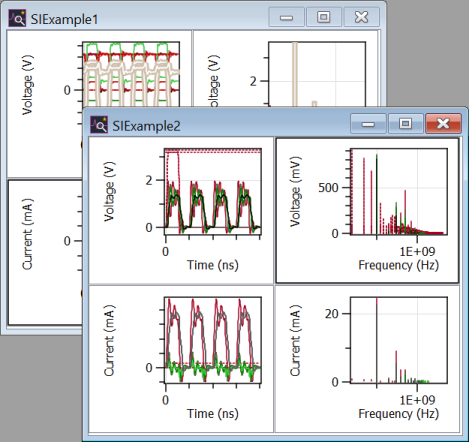
Comparing Charts
- Open
 the data sources
from the file system. For each opened data source, a new Working Set
is created and is displayed in the Working Set Area.
the data sources
from the file system. For each opened data source, a new Working Set
is created and is displayed in the Working Set Area. - Create a new Working Set
to store the relevant Probe Sets.
- Select individual probe sets from the Working Sets, and drag them into the new Working Set. Alternatively, drag them directly into the related Chart Window.
- Inspect the charts. For example, in the time and frequency domain as shown below. If required, improve the clarity of the comparison by changing the color, line and bar Attributes.
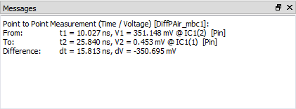
- User the Point
 or Point-to-point
 measurement to exactly measure differences.
These measurement values are displayed in the Messages
window.
measurement to exactly measure differences.
These measurement values are displayed in the Messages
window.
Working with SI Parameter Sweep Data
An SI Parameter Sweep job comprises a set of SI simulations, where one or more parameters are varied. The Data Source list shows this by providing the individual data sources, as well as a summary entry. The summary entry can be expanded or collapsed by clicking the button. The Data Source tree view shows the topology of the SI simulations with all contained pins.
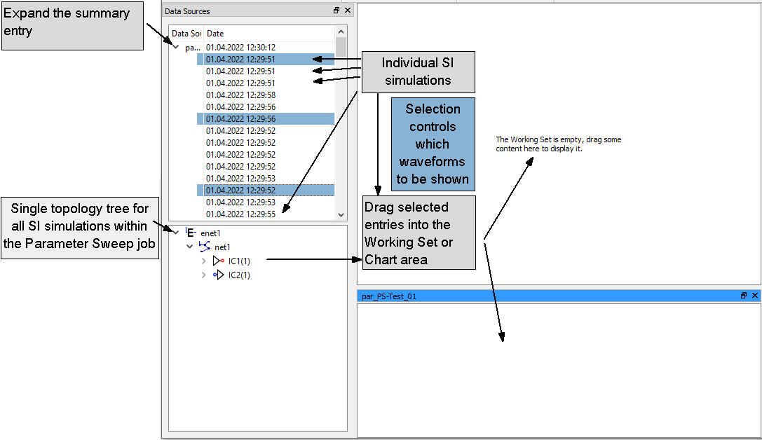
When creating a Working Set to show the waveforms, the selection in the Data Source list determines the content of the working set.
Select Summary entry
Dragging selected pins from the Data Source tree into the new Working Set automatically adds all probes of all individual SI Simulations to the working set. This allows you to compare the waveforms of selected pins across the varied parameter.
Select individual entry or entries
Dragging selected pins from the Data Source tree into the new Working Set adds a single probe to the working set. Dragging the root of the Data Source tree into the new Working Set adds all probes of the selected SI simulation to it. This is the same as in a normal SI simulation, which allows you to view all probes simultaneously, in a single view.
In an SI Parameter Sweep, the Working Set is initially not populated after loading the Data Source due to the potentially large amount of data. It is recommended to take one of the above selections.
Viewing SI Eye Pattern Data
Opening an Eye Pattern data source displays the Analysis Result Viewer in SI Eye Pattern mode. This mode provides viewing functionality that is optimized for Eye Pattern. The limitations of the SI Eye Pattern mode are listed here.
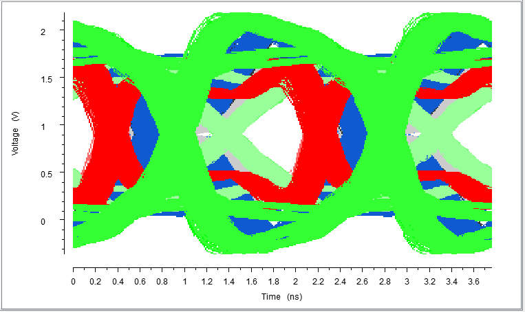
- Eye Patterns can be displayed in monochrome, where
each probe of the working set is displayed in its color, on top of
each other.
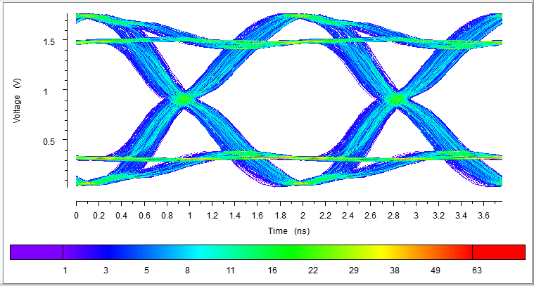
- For a single selected probe in the Working Set, a histogram view is available. This shows a more detailed statistical analysis of the Eye Pattern.
Histogram View
A single, signal probe can be visualized as a histogram plot. Each point in the voltage-time plane is colored, based on the occurrence of a voltage waveform within the unit interval at that particular location. The occurrence is mapped to a color scheme from violet (low occurrence) to red (high occurrence).
To toggle between the monochrome and histogram Eye Pattern,
click the  button on the Eye Pattern toolbar.
Measurement results for Eye Pattern are displayed for the selected base signal in the Measurements window. When you point the cursor at the histogram view, the Coordinate toolbar shows the number of waveforms at the mouse position (X,Y).

Base Signal
An Eye Pattern is essentially a folded time domain signal v(t) at a particular probe location. The folding interval is chosen to be two unit intervals (UI). To define the folding positions in time, a base signal must be specified to trigger the folding procedure.
The selected base signal probe allows you to center the Eye Pattern, and provides Eye Pattern measurement results. The Eye Patterns for all other probes are displayed relative to the base signal. Turn off this relation to the base signal by deselecting the Base Signal Trigger button in the Eye Pattern toolbar.
The Working Set indicates the currently-selected base signal by showing a modified icon that includes a "B" on the selected base signal probe. You can select the base signal by right-clicking and choosing Set Base Signal on the assist menu. Alternatively, double-click or press the B key.
Strobe Signal
A synchronous clock signal is typically used a the strobe signal to define Setup and Hold times. For example, in memory interfaces. The Strobe Signal is used in the Setup and Hold mask within the Eye Pattern.
See the Mask Editor topic for the definition of masks, and the measurement appendix for details on eye pattern measurements.
The Working Set indicates the currently-selected strobe signal, by showing a modified icon which has an "S" on the selected strobe signal probe.
- The strobe signal can be selected by right-clicking and choosing Set Strobe Signal on the assist menu. Alternatively, double-click or press the N key.
- The strobe signal can be shifted graphically within the Chart area by selecting it with the mouse. Measured values for Setup and Hold margins are updated while the signal is shifted.
SI Eye Pattern Mode Limitations
- Zooming Limitations:
since the Eye Pattern is a statistical evaluation of the time domain
signal within a fixed voltage and time range, no general zooming functionality
is supported. However, Zoom Selected
 and Display
All allow an optimal
display of the Eye Pattern within the Chart
Area window.
and Display
All allow an optimal
display of the Eye Pattern within the Chart
Area window. - Interactive Measurements: the snap mode Snap to Graphic Point is not available in the SI Eye Pattern mode.
- Available Charts: Eye Pattern diagrams are based on voltage waveforms, hence currents cannot be displayed in SI Eye Pattern mode. No frequency domain characteristics are available for the probes (no Fast Fourier Transform (FFT) can be displayed). To view the FFT, stimulus or the currents of the signal, you must perform an SI Simulation on the topology.
- CSV Export: Eye Pattern diagrams cannot be exported to CSV.
4: Miscellaneous Area
Additional windows are available in the Analysis Result Viewer. These are listed below.
Configure Eye Pattern and Eye Masks
You can arrange these as dockable windows in the main window area or outside of it, on the desktop of your PC. Initially, they are grouped in the Miscellaneous Area.
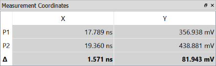
Measurement Coordinates
Interactive point or point-to-point measurements can be performed. The obtained measurement results of these user actions are listed in the Messages area, as well as the display in the Measurement Coordinates window.
Interactive measurement values are continuously shown in the Measurement Coordinates window.
The values can be copied and pasted into other applications as a table. Select Copy on the assist menu or press Ctrl+C.
Select Clear Measurements on the assist menu to remove the current display and all measure lines in the related chart. The same options are displayed by right-clicking a chart.
Measurements
The Measurements window provides measurement data which has been obtained during the SI Analysis. These values are contained in the data source file. Tabs are available for the following.
- Single pin measurements
- Pin-to-Pin measurements, where waveforms from two related pins are used to derive the measurement value.
Detailed explanations of the provided measurement results are provided in the Appendix.
Display Control of SI Measurements
Depending on the provided measurement thresholds for a buffer model, a potentially large number of different measurement results is available. These can be filtered by the following filter buttons within the measurement windows.
For Single pin measurements:

| Value | Description |
|---|---|
 Extrema Extrema
|
Toggles the display of extreme values such as topline, baseline, minimum and maximum value. |
 Ringing Ringing
|
Toggles the display of all overshoot and undershoot values, as well as settling times. |
 Edges Edges
|
Toggles the display of all rise and fall time measurements. |
 Slopes Slopes
|
Toggles the display of all slope and slew rate measurements |
 Crossings Crossings
|
This button toggles the display of crossing voltage values measured in differential pairs. |
For Pin-to-Pin measurements:

| Value | Description |
|---|---|
 Compensated
Flight Times Compensated
Flight Times
|
Toggles the display of all compensated flight times |
 Flight Times Flight Times
|
Toggles the display of all flight times. |
 Typical Flight
Times Typical Flight
Times
|
Toggles the display of typical flight times and compensated flight times. |
 Non-typical Flight
Times Non-typical Flight
Times
|
Toggles the display of the following measurements.
|
Common controls for both measurement result tables:
| Value | Description |
|---|---|
 Dynamic AC Dynamic AC
|
Toggles the display of the dynamic (ac) receiver thresholds, and their related measurement results. |
 Static DC Static DC
|
Toggles the display of the static (dc) receiver thresholds, and their related measurement results. |
 Rising Edge Rising Edge
|
Toggles the display of all rising edge related measurement results. |
 Falling Edge Falling Edge
|
Toggles the display of all falling edge related measurement results. |
 Constants Constants
|
Toggles the display of constant values such as receiver thresholds. |
| Toggles the display of empty/unpopulated measurement rows in the measurement table. It is used to shrink the table size. |
These buttons act simultaneously on both SI measurement tables.
SI Measurement tables
A separate column is used to display the measured values for each selected probe set.
Not all measurement results are available for some Pin types. In these cases, the table entries remain empty. This is particularly true for driver pins, which have no measurement data available. For example, flight time results are only available for receiver pins.
The column header provides the Component and Pin name to identify the measurement results. Further identification marks can be found in the list:
- Probe Set
- Pulse
And additionally, for Pin-to-Pin Measurements:
- Reference Ref. Pin
- Reference Ref. Location (Pin or Die)
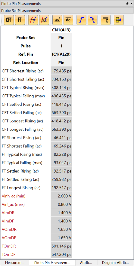
The red colored entries refer to fixed threshold values. These are derived from the buffer models, either directly or by means of a testload simulation, in the case of TOmDR/TOmDF.
The latter values are shown in the Pin-to-Pin Measurements dialog for a selected receiver pin, referencing the driver pin shown under Ref. Pin.
- You can re-order the rows and columns by dragging the header.
- To copy selected Measurements rows to the clipboard, press Ctrl+C or right-click and select Copy on the assist menu. Paste them into other applications, such as MS Excel.
- The measured data is displayed in the Measurements
panel for the selected probe set. This is illustrated below.
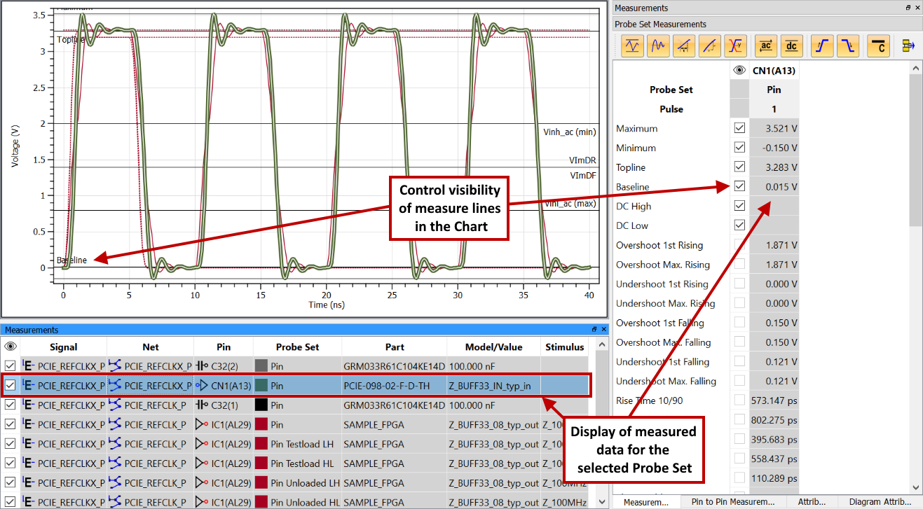
- Control the attributes of waveforms in the Attributes panel.
- Control the display of measure lines and the
label (for example, "Baseline") in the Chart by toggling
the Visibility
 check boxes for each
measured value.
check boxes for each
measured value. - When viewing measurement results for multiple pins simultaneously, you might prefer to undock the Measurements window so that you can increase its width.
- The Settings dialog allows you to control the display of measurement results simultaneously for all probe sets, or for just the selected probe set. It also allows you to control the display of thresholds and reference voltages if no actual measurement values exist. For example, when die probes are selected but only pin measurement results are available.
Eye Pattern Measurements
In SI Eye Pattern mode, measurements are performed automatically on a selected base signal probe.
This may initially take a long time on a newly-selected base signal probe.
The upper area of the measurement dialog shows the probe-related results for the selected probe in the Working Set. For details on these measurement results, see: Appendix.
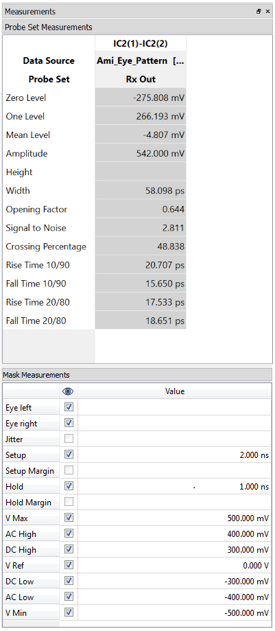
The lower area of the measurement dialog in the SI Eye Pattern mode shows measurements related to Setup and Hold, when a Setup and Hold mask is selected. These measurements depend on the selected mask and the Strobe signal. They are therefore updated when these parameters have changed.
- Where reference lines are displayed in the chart
area, you can enable and disable these using the
 Visibility check boxes, per entry.
 - Pick the strobe signal in the chart, and shift it to a suitable point in time, as needed. The Setup and Hold margin values are updated in the Mask Measurements dialog. For details on these measurement results, see: Appendix.
- 1 V for voltages
- 1 A for currents
- 1 Ω for impedances
- 1 µV/m for electric field strengths
- 1 for S-Parameter
- Select Set Custom Ranges on the assist menu in an active chart window to set this and the maximum value. This is based on the current zoom range.
- When you confirm the changes by pressing Enter, or you select another object with the mouse, the new axis range becomes effective on all diagrams of the same axis type, in the selected working set.
- Click the Custom Zoom
button
to apply the setting to all other diagrams of the same axis type
in other working sets. For example, Voltage.
- Select Set Custom Ranges on the assist menu on an active chart window to set this and the Minimum value. These settings are based on the current zoom range.
- When you press Enter, or select another object with the mouse, the new axis range becomes effective on all diagrams of the same axis type, in the selected working set.
- Click the Custom
Zoom button to apply
the setting to all other diagrams of the same axis type in other
working sets. For example, Voltage.
- Diagram attributes cannot be modified for Eye Pattern
- Custom Zoom Ranges can be used when the Base Signal Trigger is deselected.
- If Show Zero Level
is selected, then the
 Display
All,
Display
All,  Display All in All Charts and
  Zoom Selectedzoom actions contain
the zero level within the zoom range.
Zoom Selectedzoom actions contain
the zero level within the zoom range. - This function is only available when the axis Scale is set to Linear.
- You can copy selected content from the Messages window, in order to paste it into other applications for documentation purposes, for example. Do this by right-clicking and selecting Copy on the assist menu, or press Ctrl+C.
- To select all of the content, right-click and choose Select All on the assist menu or press Ctrl+A.
- To remove the content from the Messages window, right-click and choose Clear on the assist menu. Related measurement lines in the chart are also removed.
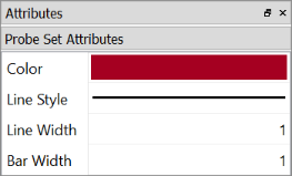
Attributes
You can control the display attributes for the probe sets in the Attributes window. The Attributes dialog contains the attributes for the probe set. These can be controlled for each probe set.
In SI Eye Pattern mode, only the color can be modified for a monochrome Eye Pattern.
| Value | Description |
|---|---|
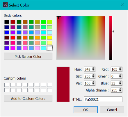
| Color |
Click on the colored cell to display the color selection dialog. Select the required color and press OK.
|
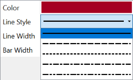
| Line Style |
Change the line style by selecting a value in the drop down menu.
|
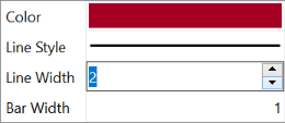
| Line Width |
Change the drawing width of lines between 1 and 10. Enter the value directly into the Line Width box, or use the "arrow" buttons. |
| Bar Width | Change the drawing width of bars between 1 and 30. Enter a value directly into the Bar Width box, or use the "arrow" buttons. |
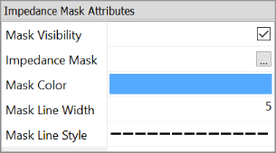
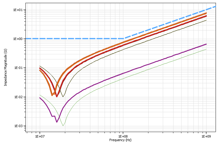
In Frequency-Domain mode: when showing Impedance plots Z(f), an impedance mask can be shown in the Chart area. Impedance Mask Attributes contains the parameters to control the display of the impedance mask and allow you to configure the mask, and its appearance.
| Value | Description |
|---|---|
| Mask Visibility | Use this checkbox to enable or disable the visibility of the selected impedance mask within the Chart area of an impedance plot. |
| Impedance Mask | Select the Impedance mask from here. The name of the selected
mask is displayed in this cell. Clicking  ,
in the Frequency-Domain mode. ,
in the Frequency-Domain mode. |
| Mask Color | Specify the color of the selected mask. A color selection dialog is displayed when you click the Color cell. |
| Mask Line Width | Select the width of the impedance mask, between 1 and 10. Enter the value directly into the editable cell, or use the small "arrow" symbols to adjust this value. |
| Mask Line Style |
Select the line style of the impedance mask. Examples are shown below.
|
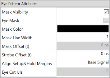
In Eye Pattern mode, additional Eye Pattern Attributes are shown in the lower part of the dialog. These allow the configuration of eye masks for the displayed eye pattern.
| Value | Description |
|---|---|
| Mask Visibility | Enable or disable the visibility of the selected eye mask within the Chart area of an eye pattern. |
| Eye Mask | Select the Standard eye mask or Setup & Hold mask
from here. The name of the selected mask is displayed
in this cell.
The Mask
Editor is opened when you press the . |
| Mask Color |
Choose the color of a selected mask. A color selection dialog is displayed when you click the color cell. |
| Mask Line Width |
Select the width of the eye mask, between 1 and 10. Enter a value in the cell, or use the "arrow" buttons. |
| Mask Offset (t) | Allows you to move the eye mask in +/- steps, in the selected unit. Allowed values are within the range of +/- 1µs. You can also type a value into the cell. Invalid entries are shown using a red background color. The Mask Editor also allows you to specify a value for the mask offset. Both values are added to adjust the mask position. |
| Strobe Offset (t) |
Allows you to move a selected strobe signal relative to the centred eye pattern display. A displayed Setup and Hold mask is placed relative to the strobe signal, if one is selected. Allowed values are within the range of +/- 1µs. You can also type a value into the cell. Invalid entries are shown using a red background color. |
| Align Setup & Hold Margins |
Always you to set whether the calculation of the Setup & Hold margins uses the eye pattern for all visible signals, or the eye pattern of just the base signal. Note
The visibility is controlled in the working set by the Visibility check boxes.
This also applies when viewing the eye pattern in Histogram
view, where only one eye pattern can be viewed at
a time. In the following example: Eye Pattern view shows two visible signal probes, which are used to determine the Setup & Hold margins. When changing the setting to the base signal, the Hold margin will extend up to the eye pattern of the green signal. This is the selected base signal probe.
|
| Eye Cut UIs |
To view more than one eye opening, set the Eye Cut UIs as an integer for the unit interval (UI), between 2 and 1000. The time axis is automatically adjusted to the new period time of the selected number of UIs. Use the Custom Zoom command to manually specify a different time range. This functionality is available when the Base Signal Trigger is deselected for SI Eye Pattern. Since AMI Eye Pattern is generated as histogram data for one eye opening, this function is not available for AMI Eye Pattern. |
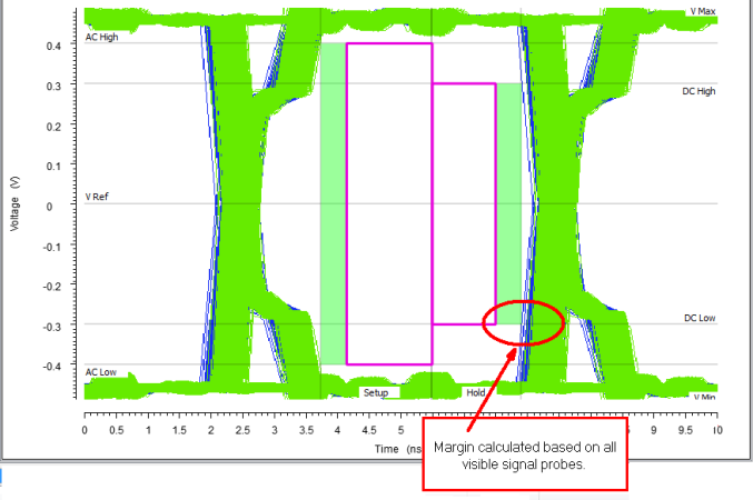
Diagram Attributes
The Diagram Attributes window allows you to control the axis scale type, axis ranges and grid lines for the different types of axis. Select a diagram to select the axis type. For example, Electric Field Strength.
The Diagram Attributes window becomes active, and the axis settings can be changed for the Electric Field Strength axis, in the selected working set. Synchronized axes like time or frequency
keep the same scale and range.
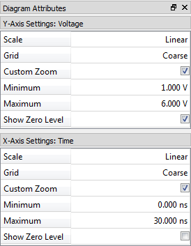
Scale
Scale allows you to toggle between a Linear scale, a dB scale and a Logarithmic scale. If you select a value, then the view of the selected axis is immediately changed.
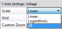
In some cases, a logarithmic or dB scale is not appropriate. For example, for time axis. In these cases, only appropriate options are available. When using a dB scale, the following reference values apply, depending on the physical quantity of the selected axis. These are:
You cannot change these reference values.
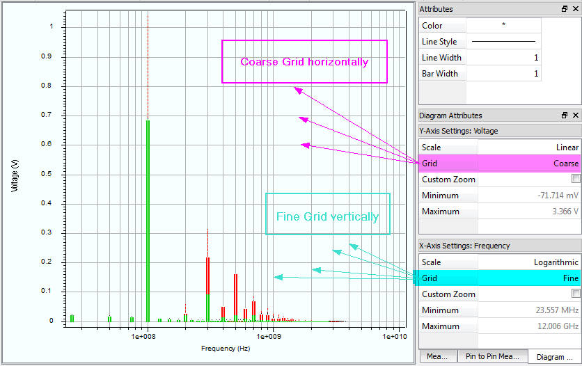
Grid
Grid allows you to display grid lines for a selected axis.
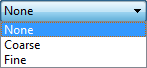
| Value | Description |
|---|---|
| None | Disables the display of grid lines. |
| Coarse | Displays grid lines at each major tick of the selected axis. |
| Fine | Displays grid lines at each major and minor tick of the selected axis. |
The following example shows grid lines in a logarithmic scaled chart.
Custom Zoom
Selecting this check box allows you to manually set the axis range in the selected diagram. The entries for Minimum and Maximum are made available.
If you select Custom Zoom
within
all Working Sets, then all axes are considered.Minimum
Minimum allows you to control the lower axis range. This parameter is available separately for the Linear and Logarithmic scale. When the editor is opened, the value and the unit can be entered separately.
Maximum
Maximum allows you to control the upper axis range. This parameter is available separately for the Linear and Logarithmic scale. When the editor is opened, the value and the unit can be entered separately.
Show Zero Level
Selecting this check box for the x axis or y axis on a selected diagram ensures that the respective zero level is included in the diagram. This may help to compare charts.
Custom Zoom ranges that are set have priority over this setting. This means that if you select the Custom Zoom
button, then the user-defined ranges are applied, regardless of this
setting.AMI Parameters
The dockable AMI Parameters window allows you to view the used AMI Parameters that are derived from the AMI Simulation process. You can review the used AMI Parameters using the same functionality as the full AMI Parameters utility.
| Value | Description | |
|---|---|---|
| Summary | Provides the name and a description of the AMI file, and the selected parameter set | |
| Name | Provides the name of the AMI file. | |
| Description | Provides a description of the AMI file. | |
| Parameter Set | The name of the parameter set that is used. Parameters which have been modified by the AMI runtime library during the AMI Simulation process are indicated with a red background color. | |
| Filter | Filter buttons allows you to reduce the number of items
that are shown in the tree view.
 A text filter provides a more detailed way to narrow down the displayed parameters. Previously-used text filter entries can be re-used by clicking the "arrow" button. |
|

|
Resets all filter settings. |
A read-only version of the AMI
Parameters dialog can be launched from the working set on a selected
AMI probe set. Do this by selecting it on the assist menu or by a
clicking ![]() . For more details, see: AMI
Parameters.
. For more details, see: AMI
Parameters.
Messages
The Messages window displays any messages that are generated by the Analysis Result Viewer. Its main purpose is to display the measurement values that are obtained during interactive point or point-to-point measurements.